Attention mechanisms

Acknowledgement

Most of the information in this blog post is sourced from Machine Learning Mastery.

Also read All you need to know about ‘Attention’ and ‘Transformers’ — In-depth Understanding — Part 1 and All you need to know about ‘Attention’ and ‘Transformers’ — In-depth Understanding — Part 2.

The Attention Mechanism from Scratch

By Stefania Cristina on January 6, 2023 in Attention 27

The attention mechanism was introduced to improve the performance of the encoder-decoder model for machine translation. The idea behind the attention mechanism was to permit the decoder to utilize the most relevant parts of the input sequence in a flexible manner, by a weighted combination of all the encoded input vectors, with the most relevant vectors being attributed the highest weights. 

After completing this tutorial, you will know:

• How the attention mechanism uses a weighted sum of all the encoder hidden states to flexibly focus the attention of the decoder on the most relevant parts of the input sequence
• How the attention mechanism can be generalized for tasks where the information may not necessarily be related in a sequential fashion
• How to implement the general attention mechanism in Python with NumPy and SciPy 

The Attention Mechanism

The attention mechanism was introduced by Bahdanau et al. (2014) to address the bottleneck problem that arises with the use of a fixed-length encoding vector, where the decoder would have limited access to the information provided by the input. This is thought to become especially problematic for long and/or complex sequences, where the dimensionality of their representation would be forced to be the same as for shorter or simpler sequences.

Note that Bahdanau et al.’s attention mechanism is divided into the step-by-step computations of the alignment scores, the weights, and the context vector:

1. Alignment scores: The alignment model takes the encoded hidden states, ${\mathbf{h}}_i$, and the previous decoder output, ${\mathbf{s}}_{t-1}$, to compute a score, $e_{t,i}$, that indicates how well the elements of the input sequence align with the current output at the position, $t$. The alignment model is represented by a function, $a(.)$, which can be implemented by a feedforward neural network:

$$e_{t,i}=a({\mathbf{s}}_{t-1},{\mathbf{h}}_i)$$

2. Weights: The weights, ${\alpha }_{t,i}$, are computed by applying a softmax operation to the previously computed alignment scores:

$${\alpha }_{t,i}=\text{softmax}(e_{t,i})$$

3. Context vector: A unique context vector, ${\mathbf{c}}_t$, is fed into the decoder at each time step. It is computed by a weighted sum of all, $T$, encoder hidden states:

$${\mathbf{c}}_t=\sum _{i=1}^T{\alpha }_{t,i}{\mathbf{h}}_i$$

Bahdanau et al. implemented an RNN for both the encoder and decoder. 

However, the attention mechanism can be re-formulated into a general form that can be applied to any sequence-to-sequence (abbreviated to seq2seq) task, where the information may not necessarily be related in a sequential fashion. 

In other words, the database doesn’t have to consist of the hidden RNN states at different steps, but could contain any kind of information instead.

– Advanced Deep Learning with Python, 2019.

The General Attention Mechanism

The general attention mechanism makes use of three main components, namely the queries, $\mathbf{Q}$, the keys, $\mathbf{K}$, and the values, $\mathbf{V}$. 

If you had to compare these three components to the attention mechanism as proposed by Bahdanau et al., then the query would be analogous to the previous decoder output, ${\mathbf{s}}_{t-1}$, while the values would be analogous to the encoded inputs, ${\mathbf{h}}_i$. In the Bahdanau attention mechanism, the keys and values are the same vector.

In this case, we can think of the vector ${\mathbf{s}}_{t-1}$ as a query executed against a database of key-value pairs, where the keys are vectors and the hidden states ${\mathbf{h}}_i$ are the values.

– Advanced Deep Learning with Python, 2019.

The general attention mechanism then performs the following computations:

1. Each query vector, $\mathbf{q}={\mathbf{s}}_{t-1}$, is matched against a database of keys to compute a score value. This matching operation is computed as the dot product of the specific query under consideration with each key vector, ${\mathbf{k}}_i$: 

$$e_{\mathbf{q},{\mathbf{k}}_i}=\mathbf{q}\cdot {\mathbf{k}}_i$$

2. The scores are passed through a softmax operation to generate the weights:

$${\alpha }_{\mathbf{q},{\mathbf{k}}_i}=\text{softmax}(e_{\mathbf{q},{\mathbf{k}}_i})$$

3. The generalized attention is then computed by a weighted sum of the value vectors, ${\mathbf{v}}_{{\mathbf{k}}_i}$, where each value vector is paired with a corresponding key:

$$\text{attention}(\mathbf{q},\mathbf{K},\mathbf{V})=\sum _i{\alpha }_{\mathbf{q},{\mathbf{k}}_i}{\mathbf{v}}_{{\mathbf{k}}_i}$$

Within the context of machine translation, each word in an input sentence would be attributed its own query, key, and value vectors. These vectors are generated by multiplying the encoder’s representation of the specific word under consideration with three different weight matrices that would have been generated during training. 

In essence, when the generalized attention mechanism is presented with a sequence of words, it takes the query vector attributed to some specific word in the sequence and scores it against each key in the database. In doing so, it captures how the word under consideration relates to the others in the sequence. Then it scales the values according to the attention weights (computed from the scores) to retain focus on those words relevant to the query. In doing so, it produces an attention output for the word under consideration. 

The Bahdanau Attention Mechanism

Conventional encoder-decoder architectures for machine translation encoded every source sentence into a fixed-length vector, regardless of its length, from which the decoder would then generate a translation. This made it difficult for the neural network to cope with long sentences, essentially resulting in a performance bottleneck. 

The Bahdanau attention was proposed to address the performance bottleneck of conventional encoder-decoder architectures, achieving significant improvements over the conventional approach. 

In this tutorial, you will discover the Bahdanau attention mechanism for neural machine translation. 

After completing this tutorial, you will know:

• Where the Bahdanau attention derives its name from and the challenge it addresses
• The role of the different components that form part of the Bahdanau encoder-decoder architecture
• The operations performed by the Bahdanau attention algorithm

Tutorial Overview

This tutorial is divided into two parts; they are:

• Introduction to the Bahdanau Attention
• The Bahdanau Architecture
  • The Encoder
  • The Decoder
  • The Bahdanau Attention Algorithm

Prerequisites

For this tutorial, we assume that you are already familiar with:

• Recurrent Neural Networks (RNNs)
• The encoder-decoder RNN architecture
• The concept of attention
• The attention mechanism

Introduction to the Bahdanau Attention

The Bahdanau attention mechanism inherited its name from the first author of the paper in which it was published. 

It follows the work of Cho et al. (2014) and Sutskever et al. (2014), who also employed an RNN encoder-decoder framework for neural machine translation, specifically by encoding a variable-length source sentence into a fixed-length vector. The latter would then be decoded into a variable-length target sentence. 

Bahdanau et al. (2014) argued that this encoding of a variable-length input into a fixed-length vector squashes the information of the source sentence, irrespective of its length, causing the performance of a basic encoder-decoder model to deteriorate rapidly with an increasing length of the input sentence. The approach they proposed replaces the fixed-length vector with a variable-length one to improve the translation performance of the basic encoder-decoder model. 

The most important distinguishing feature of this approach from the basic encoder-decoder is that it does not attempt to encode a whole input sentence into a single fixed-length vector. Instead, it encodes the input sentence into a sequence of vectors and chooses a subset of these vectors adaptively while decoding the translation.

– Neural Machine Translation by Jointly Learning to Align and Translate, 2014.

The Bahdanau Architecture

The main components in use by the Bahdanau encoder-decoder architecture are the following:

• ${\mathbf{s}}_{t-1}$ is the hidden decoder state at the previous time step, $t-1$.
• ${\mathbf{c}}_t$ is the context vector at time step, $t$. It is uniquely generated at each decoder step to generate a target word, $y_t$.
• ${\mathbf{h}}_i$ is an annotation that captures the information contained in the words forming the entire input sentence, $\{x_1,x_2,\dots ,x_T\}$, with strong focus around the $i$-th word out of $T$ total words. 
• ${\alpha }_{t,i}$ is a weight value assigned to each annotation, ${\mathbf{h}}_i$, at the current time step, $t$.
• $e_{t,i}$ is an attention score generated by an alignment model, $a(.)$, that scores how well ${\mathbf{s}}_{t-1}$ and ${\mathbf{h}}_i$ match.

These components find their use at different stages of the Bahdanau architecture, which employs a bidirectional RNN as an encoder and an RNN decoder, with an attention mechanism in between:

The Bahdanau architecture

The Encoder

The role of the encoder is to generate an annotation, ${\mathbf{h}}_i$, for every word, $x_i$, in an input sentence of length $T$ words. 

For this purpose, Bahdanau et al. employ a bidirectional RNN, which reads the input sentence in the forward direction to produce a forward hidden state, $\overrightarrow{{\mathbf{h}}_i}$, and then reads the input sentence in the reverse direction to produce a backward hidden state, $\overleftarrow{{\mathbf{h}}_i}$. The annotation for some particular word, $x_i$, concatenates the two states:

$${\mathbf{h}}_i={[\overrightarrow{{\mathbf{h}}_i^T};\overleftarrow{{\mathbf{h}}_i^T}]}^T$$

The idea behind generating each annotation in this manner was to capture a summary of both the preceding and succeeding words. 

In this way, the annotation ${\mathbf{h}}_i$ contains the summaries of both the preceding words and the following words.

– Neural Machine Translation by Jointly Learning to Align and Translate, 2014.

The generated annotations are then passed to the decoder to generate the context vector. 

The Decoder

The role of the decoder is to produce the target words by focusing on the most relevant information contained in the source sentence. For this purpose, it makes use of an attention mechanism. 

Each time the proposed model generates a word in a translation, it (soft-)searches for a set of positions in a source sentence where the most relevant information is concentrated. The model then predicts a target word based on the context vectors associated with these source positions and all the previous generated target words.

– Neural Machine Translation by Jointly Learning to Align and Translate, 2014.

The decoder takes each annotation and feeds it to an alignment model, $a(.)$, together with the previous hidden decoder state, ${\mathbf{s}}_{t-1}$. This generates an attention score:

$$e_{t,i}=a({\mathbf{s}}_{t-1},{\mathbf{h}}_i)$$

The function implemented by the alignment model here combines ${\mathbf{s}}_{t-1}$ and ${\mathbf{h}}_i$ using an addition operation. For this reason, the attention mechanism implemented by Bahdanau et al. is referred to as additive attention.

This can be implemented in two ways, either (1) by applying a weight matrix, $\mathbf{W}$, over the concatenated vectors, ${\mathbf{s}}_{t-1}$ and ${\mathbf{h}}_i$, or (2) by applying the weight matrices, ${\mathbf{W}}_1$ and ${\mathbf{W}}_2$, to ${\mathbf{s}}_{t-1}$ and ${\mathbf{h}}_i$ separately:

1. $$a({\mathbf{s}}_{t-1},{\mathbf{h}}_i)={\mathbf{v}}^T\tanh (\mathbf{W}[{\mathbf{h}}_i;{\mathbf{s}}_{t-1}])$$
2. $$a({\mathbf{s}}_{t-1},{\mathbf{h}}_i)={\mathbf{v}}^T\tanh ({\mathbf{W}}_1{\mathbf{h}}_i+{\mathbf{W}}_2{\mathbf{s}}_{t-1})$$

Here, $\mathbf{v}$ is a weight vector. 

The alignment model is parametrized as a feedforward neural network and jointly trained with the remaining system components. 

Subsequently, a softmax function is applied to each attention score to obtain the corresponding weight value:

$${\alpha }_{t,i}=\text{softmax}(e_{t,i})$$

The application of the softmax function essentially normalizes the annotation values to a range between 0 and 1; hence, the resulting weights can be considered probability values. Each probability (or weight) value reflects how important ${\mathbf{h}}_i$ and ${\mathbf{s}}_{t-1}$ are in generating the next state, ${\mathbf{s}}_t$, and the next output, $y_t$.

Intuitively, this implements a mechanism of attention in the decoder. The decoder decides parts of the source sentence to pay attention to. By letting the decoder have an attention mechanism, we relieve the encoder from the burden of having to encode all information in the source sentence into a fixed-length vector.

– Neural Machine Translation by Jointly Learning to Align and Translate, 2014.

This is finally followed by the computation of the context vector as a weighted sum of the annotations:

$${\mathbf{c}}_t=\sum _{i=1}^T{\alpha }_{t,i}{\mathbf{h}}_i$$

The Bahdanau Attention Algorithm

In summary, the attention algorithm proposed by Bahdanau et al. performs the following operations:

1. The encoder generates a set of annotations, ${\mathbf{h}}_i$, from the input sentence. 
2. These annotations are fed to an alignment model and the previous hidden decoder state. The alignment model uses this information to generate the attention scores, $e_{t,i}$. 
3. A softmax function is applied to the attention scores, effectively normalizing them into weight values, ${\alpha }_{t,i}$, in a range between 0 and 1.  
4. Together with the previously computed annotations, these weights are used to generate a context vector, ${\mathbf{c}}_t$, through a weighted sum of the annotations. 
5. The context vector is fed to the decoder together with the previous hidden decoder state and the previous output to compute the final output, $y_t$. 
6. Steps 2-6 are repeated until the end of the sequence. 

Bahdanau et al. tested their architecture on the task of English-to-French translation. They reported that their model significantly outperformed the conventional encoder-decoder model, regardless of the sentence length. 

There have been several improvements over the Bahdanau attention proposed, such as those of Luong et al. (2015), which we shall review in a separate tutorial. 

Further Reading

• Advanced Deep Learning with Python, 2019.
• Neural Machine Translation by Jointly Learning to Align and Translate, 2014.

The Luong Attention Mechanism

The Luong attention sought to introduce several improvements over the Bahdanau model for neural machine translation, notably by introducing two new classes of attentional mechanisms: a global approach that attends to all source words and a local approach that only attends to a selected subset of words in predicting the target sentence. 

Prerequisites

For this tutorial, we assume that you are already familiar with:

• The concept of attention
• The attention mechanism
• The Bahdanau attention mechanism

Introduction to the Luong Attention

Luong et al. (2015) inspire themselves from previous attention models to propose two attention mechanisms:

In this work, we design, with simplicity and effectiveness in mind, two novel types of attention-based models: a global approach which always attends to all source words and a local one that only looks at a subset of source words at a time.

– Effective Approaches to Attention-based Neural Machine Translation, 2015.

The global attentional model resembles the Bahdanau et al. (2014) model in attending to all source words but aims to simplify it architecturally. 

The local attentional model is inspired by the hard and soft attention models of Xu et al. (2016) and attends to only a few of the source positions. 

The two attentional models share many of the steps in their prediction of the current word but differ mainly in their computation of the context vector.

Let’s first take a look at the overarching Luong attention algorithm and then delve into the differences between the global and local attentional models afterward. 

The Luong Attention Algorithm

The attention algorithm of Luong et al. performs the following operations:

1. The encoder generates a set of annotations, $H={\mathbf{h}}_i,i=1,\dots ,T$, from the input sentence. 

2. The current decoder hidden state is computed as: ${\mathbf{s}}_t={\text{RNN}}_{\text{decoder}}({\mathbf{s}}_{t-1},y_{t-1})$. Here, ${\mathbf{s}}_{t-1}$ denotes the previous hidden decoder state and $y_{t-1}$ the previous decoder output. 

3. An alignment model, $a(.)$, uses the annotations and the current decoder hidden state to compute the alignment scores: $e_{t,i}=a({\mathbf{s}}_t,{\mathbf{h}}_i)$. 

4. A softmax function is applied to the alignment scores, effectively normalizing them into weight values in a range between 0 and 1: ${\alpha }_{t,i}=\text{softmax}(e_{t,i})$.

5. Together with the previously computed annotations, these weights are used to generate a context vector through a weighted sum of the annotations: ${\mathbf{c}}_t=\sum _{i=1}^T{\alpha }_{t,i}{\mathbf{h}}_i$. 

6. An attentional hidden state is computed based on a weighted concatenation of the context vector and the current decoder hidden state: ${\tilde{\mathbf{s}}}_t=\tanh ({\mathbf{W}}_{\mathbf{c}}[{\mathbf{c}}_t;{\mathbf{s}}_t])$.

7. The decoder produces a final output by feeding it a weighted attentional hidden state: $y_t=\text{softmax}({\mathbf{W}}_y{\tilde{\mathbf{s}}}_t)$. 

8. Steps 2-7 are repeated until the end of the sequence. 

The Global Attentional Model

The global attentional model considers all the source words in the input sentence when generating the alignment scores and, eventually, when computing the context vector. 

The idea of a global attentional model is to consider all the hidden states of the encoder when deriving the context vector, ${\mathbf{c}}_t$.

– Effective Approaches to Attention-based Neural Machine Translation, 2015.

In order to do so, Luong et al. propose three alternative approaches for computing the alignment scores. The first approach is similar to Bahdanau’s. It is based upon the concatenation of ${\mathbf{s}}_t$ and ${\mathbf{h}}_i$, while the second and third approaches implement multiplicative attention (in contrast to Bahdanau’s additive attention):

1. $$a({\mathbf{s}}_t,{\mathbf{h}}_i)={\mathbf{v}}_a^T\tanh ({\mathbf{W}}_a[{\mathbf{s}}_t;{\mathbf{h}}_i)]$$

2. $$a({\mathbf{s}}_t,{\mathbf{h}}_i)={\mathbf{s}}_t^T{\mathbf{h}}_i$$

3. $$a({\mathbf{s}}_t,{\mathbf{h}}_i)={\mathbf{s}}_t^T{\mathbf{W}}_a{\mathbf{h}}_i$$

Here, ${\mathbf{W}}_a$ is a trainable weight matrix, and similarly, ${\mathbf{v}}_a$ is a weight vector.

Intuitively, the use of the dot product in multiplicative attention can be interpreted as providing a similarity measure between the vectors, ${\mathbf{s}}_t$ and ${\mathbf{h}}_i$, under consideration. 

… if the vectors are similar (that is, aligned), the result of the multiplication will be a large value and the attention will be focused on the current t,i relationship.

– Advanced Deep Learning with Python, 2019.

The resulting alignment vector, ${\mathbf{e}}_t$, is of a variable length according to the number of source words. 

The Local Attentional Model

In attending to all source words, the global attentional model is computationally expensive and could potentially become impractical for translating longer sentences. 

The local attentional model seeks to address these limitations by focusing on a smaller subset of the source words to generate each target word. In order to do so, it takes inspiration from the hard and soft attention models of the image caption generation work of Xu et al. (2016):

• Soft attention is equivalent to the global attention approach, where weights are softly placed over all the source image patches. Hence, soft attention considers the source image in its entirety. 

• Hard attention attends to a single image patch at a time.

The local attentional model of Luong et al. generates a context vector by computing a weighted average over the set of annotations, ${\mathbf{h}}_i$, within a window centered over an aligned position, $p_t$:

$$[p_t–D,p_t+D]$$

While a value for $D$ is selected empirically, Luong et al. consider two approaches in computing a value for $p_t$:

1. Monotonic alignment: where the source and target sentences are assumed to be monotonically aligned and, hence, $p_t=t$.

2. Predictive alignment: where a prediction of the aligned position is based upon trainable model parameters, ${\mathbf{W}}_p$ and ${\mathbf{v}}_p$, and the source sentence length, $S$:

$$p_t=S\cdot \text{sigmoid}({\mathbf{v}}_p^T\tanh ({\mathbf{W}}_p,{\mathbf{s}}_t))$$

A Gaussian distribution is centered around $p_t$ when computing the alignment weights to favor source words nearer to the window center. 

This time round, the resulting alignment vector, ${\mathbf{e}}_t$, has a fixed length of $2D+1$.

Comparison to the Bahdanau Attention

The Bahdanau model and the global attention approach of Luong et al. are mostly similar, but there are key differences between the two:

While our global attention approach is similar in spirit to the model proposed by Bahdanau et al. (2015), there are several key differences which reflect how we have both simplified and generalized from the original model.

– Effective Approaches to Attention-based Neural Machine Translation, 2015.

1. Most notably, the computation of the alignment scores, $e_t$, in the Luong global attentional model depends on the current decoder hidden state, ${\mathbf{s}}_t$, rather than on the previous hidden state, ${\mathbf{s}}_{t-1}$, as in the Bahdanau attention. 

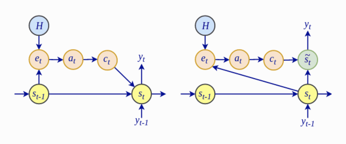
The Bahdanau architecture (left) vs. the Luong architecture (right)

2. Luong et al. drop the bidirectional encoder used by the Bahdanau model and instead utilize the hidden states at the top LSTM layers for both the encoder and decoder. 

3. The global attentional model of Luong et al. investigates the use of multiplicative attention as an alternative to the Bahdanau additive attention. 

Further Reading

• Advanced Deep Learning with Python, 2019.
• Effective Approaches to Attention-based Neural Machine Translation, 2015.

The Transformer Attention Mechanism

Before the introduction of the Transformer model, the use of attention for neural machine translation was implemented by RNN-based encoder-decoder architectures. The Transformer model revolutionized the implementation of attention by dispensing with recurrence and convolutions and, alternatively, relying solely on a self-attention mechanism.

We will first focus on the Transformer attention mechanism in this tutorial and subsequently review the Transformer model in a separate one. 

In this tutorial, you will discover the Transformer attention mechanism for neural machine translation. 

After completing this tutorial, you will know:

• How the Transformer attention differed from its predecessors
• How the Transformer computes a scaled-dot product attention
• How the Transformer computes multi-head attention

For this tutorial, we assume that you are already familiar with:

• The concept of attention
• The attention mechanism
• The Bahdanau attention mechanism
• The Luong attention mechanism

Introduction to the Transformer Attention

Thus far, you have familiarized yourself with using an attention mechanism in conjunction with an RNN-based encoder-decoder architecture. Two of the most popular models that implement attention in this manner have been those proposed by Bahdanau et al. (2014) and Luong et al. (2015). 

The Transformer architecture revolutionized the use of attention by dispensing with recurrence and convolutions, on which the formers had extensively relied. 

… the Transformer is the first transduction model relying entirely on self-attention to compute representations of its input and output without using sequence-aligned RNNs or convolution.

– Attention Is All You Need, 2017.

In their paper, “Attention Is All You Need,” Vaswani et al. (2017) explain that the Transformer model, alternatively, relies solely on the use of self-attention, where the representation of a sequence (or sentence) is computed by relating different words in the same sequence. 

Self-attention, sometimes called intra-attention, is an attention mechanism relating different positions of a single sequence in order to compute a representation of the sequence.

– Attention Is All You Need, 2017.

The Transformer Attention

The main components used by the Transformer attention are the following:

• $\mathbf{q}$ and $\mathbf{k}$ denoting vectors of dimension, $d_k$, containing the queries and keys, respectively
• $\mathbf{v}$ denoting a vector of dimension, $d_v$, containing the values
• $\mathbf{Q}$, $\mathbf{K}$, and $\mathbf{V}$ denoting matrices packing together sets of queries, keys, and values, respectively.
• ${\mathbf{W}}^Q$, ${\mathbf{W}}^K$ and ${\mathbf{W}}^V$ denoting projection matrices that are used in generating different subspace representations of the query, key, and value matrices
• ${\mathbf{W}}^O$ denoting a projection matrix for the multi-head output

In essence, the attention function can be considered a mapping between a query and a set of key-value pairs to an output. 

The output is computed as a weighted sum of the values, where the weight assigned to each value is computed by a compatibility function of the query with the corresponding key.

– Attention Is All You Need, 2017.

Vaswani et al. propose a scaled dot-product attention and then build on it to propose multi-head attention. Within the context of neural machine translation, the query, keys, and values that are used as inputs to these attention mechanisms are different projections of the same input sentence. 

Intuitively, therefore, the proposed attention mechanisms implement self-attention by capturing the relationships between the different elements (in this case, the words) of the same sentence. 

Scaled Dot-Product Attention

The Transformer implements a scaled dot-product attention, which follows the procedure of the general attention mechanism that you had previously seen. 

As the name suggests, the scaled dot-product attention first computes a dot product for each query, $\mathbf{q}$, with all of the keys, $\mathbf{k}$. It subsequently divides each result by $\sqrt{d_k}$ and proceeds to apply a softmax function. In doing so, it obtains the weights that are used to scale the values, $\mathbf{v}$.

Scaled dot-product attention (Taken from “Attention Is All You Need“)

In practice, the computations performed by the scaled dot-product attention can be efficiently applied to the entire set of queries simultaneously. In order to do so, the matrices—$\mathbf{Q}$, $\mathbf{K}$, and $\mathbf{V}$—are supplied as inputs to the attention function:

$$\text{attention}(\mathbf{Q},\mathbf{K},\mathbf{V})=\text{softmax}\left(\frac{Q{K}^T}{\sqrt{d_k}}\right)V$$

Vaswani et al. explain that their scaled dot-product attention is identical to the multiplicative attention of Luong et al. (2015), except for the added scaling factor of $\frac{1}{\sqrt{d_k}}$. 

This scaling factor was introduced to counteract the effect of having the dot products grow large in magnitude for large values of $d_k$, where the application of the softmax function would then return extremely small gradients that would lead to the infamous vanishing gradients problem. The scaling factor, therefore, serves to pull the results generated by the dot product multiplication down, preventing this problem. 

Vaswani et al. further explain that their choice of opting for multiplicative attention instead of the additive attention of Bahdanau et al. (2014) was based on the computational efficiency associated with the former. 

… dot-product attention is much faster and more space-efficient in practice since it can be implemented using highly optimized matrix multiplication code.

– Attention Is All You Need, 2017.

Therefore, the step-by-step procedure for computing the scaled-dot product attention is the following:

1. Compute the alignment scores by multiplying the set of queries packed in the matrix, $\mathbf{Q}$, with the keys in the matrix, $\mathbf{K}$. If the matrix, $\mathbf{Q}$, is of the size $m\times d_k$, and the matrix, $\mathbf{K}$, is of the size, $n\times d_k$, then the resulting matrix will be of the size $m\times n$:

$${\mathbf{QK}}^T=\left[\begin{array}{cccc}{e}_{11}& e_{12}& \dots & e_{1n}\\ e_{21}& e_{22}& \dots & e_{2n}\\ ⋮& ⋮& \ddots & ⋮\\ e_{m1}& e_{m2}& \dots & e_{mn}\end{array}\right]$$

2. Scale each of the alignment scores by $\frac{1}{\sqrt{d_k}}$:

$$\frac{{\mathbf{QK}}^T}{\sqrt{d_k}}=\left[\begin{array}{cccc}\frac{e_{11}}{\sqrt{d_k}}& \frac{e_{12}}{\sqrt{d_k}}& \dots & \frac{e_{1n}}{\sqrt{d_k}}\\ \frac{e_{21}}{\sqrt{d_k}}& \frac{e_{22}}{\sqrt{d_k}}& \dots & \frac{e_{2n}}{\sqrt{d_k}}\\ ⋮& ⋮& \ddots & ⋮\\ \frac{e_{m1}}{\sqrt{d_k}}& \frac{e_{m2}}{\sqrt{d_k}}& \dots & \frac{e_{mn}}{\sqrt{d_k}}\end{array}\right]$$

3. And follow the scaling process by applying a softmax operation in order to obtain a set of weights:

$$\text{softmax}\left(\frac{{\mathbf{QK}}^T}{\sqrt{d_k}}\right)=\left[\begin{array}{cccc}\text{softmax}(\frac{e_{11}}{\sqrt{d_k}}& \frac{e_{12}}{\sqrt{d_k}}& \dots & \frac{e_{1n}}{\sqrt{d_k}})\\ \text{softmax}(\frac{e_{21}}{\sqrt{d_k}}& \frac{e_{22}}{\sqrt{d_k}}& \dots & \frac{e_{2n}}{\sqrt{d_k}})\\ ⋮& ⋮& \ddots & ⋮\\ \text{softmax}(\frac{e_{m1}}{\sqrt{d_k}}& \frac{e_{m2}}{\sqrt{d_k}}& \dots & \frac{e_{mn}}{\sqrt{d_k}})\end{array}\right]$$

4. Finally, apply the resulting weights to the values in the matrix, $\mathbf{V}$, of the size, $n\times d_v$:

$$\begin{array}{rl}& \text{softmax}\left(\frac{{\mathbf{QK}}^T}{\sqrt{d_k}}\right)\cdot \mathbf{V}\\ =& \left[\begin{array}{cccc}\text{softmax}(\frac{e_{11}}{\sqrt{d_k}}& \frac{e_{12}}{\sqrt{d_k}}& \dots & \frac{e_{1n}}{\sqrt{d_k}})\\ \text{softmax}(\frac{e_{21}}{\sqrt{d_k}}& \frac{e_{22}}{\sqrt{d_k}}& \dots & \frac{e_{2n}}{\sqrt{d_k}})\\ ⋮& ⋮& \ddots & ⋮\\ \text{softmax}(\frac{e_{m1}}{\sqrt{d_k}}& \frac{e_{m2}}{\sqrt{d_k}}& \dots & \frac{e_{mn}}{\sqrt{d_k}})\end{array}\right]\cdot \left[\begin{array}{cccc}{v}_{11}& v_{12}& \dots & v_{1d_v}\\ v_{21}& v_{22}& \dots & v_{2d_v}\\ ⋮& ⋮& \ddots & ⋮\\ v_{n1}& v_{n2}& \dots & v_{n{d}_v}\end{array}\right]\end{array}$$

Multi-Head Attention

Building on their single attention function that takes matrices, $\mathbf{Q}$, $\mathbf{K}$, and $\mathbf{V}$, as input, as you have just reviewed, Vaswani et al. also propose a multi-head attention mechanism.

Their multi-head attention mechanism linearly projects the queries, keys, and values $h$ times, using a different learned projection each time. The single attention mechanism is then applied to each of these $h$ projections in parallel to produce $h$ outputs, which, in turn, are concatenated and projected again to produce a final result.

Multi-head attention (Taken from “Attention Is All You Need“)

The idea behind multi-head attention is to allow the attention function to extract information from different representation subspaces, which would otherwise be impossible with a single attention head. 

The multi-head attention function can be represented as follows:

$$\text{multihead}(\mathbf{Q},\mathbf{K},\mathbf{V})=\text{concat}({\text{head}}_1,\dots ,{\text{head}}_h){\mathbf{W}}^O$$

Here, each ${\text{head}}_i$, $i=1,\dots ,h$, implements a single attention function characterized by its own learned projection matrices:

$${\text{head}}_i=\text{attention}({\mathbf{QW}}_i^Q,{\mathbf{KW}}_i^K,{\mathbf{VW}}_i^V)$$

The step-by-step procedure for computing multi-head attention is, therefore, the following:

1. Compute the linearly projected versions of the queries, keys, and values through multiplication with the respective weight matrices, ${\mathbf{W}}_i^Q$, ${\mathbf{W}}_i^K$, and ${\mathbf{W}}_i^V$, one for each ${\text{head}}_i$.

2. Apply the single attention function for each head by (1) multiplying the queries and keys matrices, (2) applying the scaling and softmax operations, and (3) weighting the values matrix to generate an output for each head. 

3. Concatenate the outputs of the heads, ${\text{head}}_i$, $i=1,\dots ,h$.

4. Apply a linear projection to the concatenated output through multiplication with the weight matrix, ${\mathbf{W}}^O$, to generate the final result.

Further Reading
Advanced Deep Learning with Python, 2019.
Attention Is All You Need, 2017
Neural Machine Translation by Jointly Learning to Align and Translate, 2014.
Effective Approaches to Attention-based Neural Machine Translation, 2015.

 

 

Neural networks - Tutorials, examples and more reading

• Understanding RNN and LSTM
• How to choose an activation function for deep learning
• Hyperparameter optimization with random search and grid search
  

Basic statistics - Some notes and proofs

Sample variance estimation formula: Why is (n-1) to be used instead of n as the denominator?

Let Y₁, Y₂, .., Y_n be the sample data points for the random variable Y. Let μ_Y and σ_Y denote the mean and standard deviation of Y respectively. This assumption usually holds true in case of sampling with replacement. Hence, E(Y_iY_j) = E(Y_i)E(Y_j) for any i, j ∈ {1, .., n} such that i ≠ j.

The estimator for mean of Y is simply the average value of the data points, i.e. 

Mean_est(Y) or Ỹ_est =

which seems intuitive. By the same reasoning, it would seem that the best estimate for the variance of Y would be Var_est(Y) =

Let us estimate the mean value of the estimated variance, since the estimate itself is a random variable dependent on the values of data points Y_i in the sample set. Let A denote the variance estimator that uses n as the denominator. Let us denote by S_n the numerator in the formula for Ỹ_est, i.e.

Now, by definition,

Thus, the estimated variance has a mean value that is less than the actual variance. From equation ⑤, it is clear that if the estimator A is multiplied by n/(n - 1) (which is a linear transformation of A), then the resulting estimator A_mod will have a mean value that equals the actual variance. Thus, the more precise estimator of variance is: